Plotting
All of the optimization functions in EfficientFrontier produce a single optimal portfolio.
However, you may want to plot the entire efficient frontier. This efficient frontier can be thought
of in several different ways:
- The set of all
efficient_risk()portfolios for a range of target risks - The set of all
efficient_return()portfolios for a range of target returns - The set of all
max_quadratic_utility()portfolios for a range of risk aversions.
The plotting module provides support for all three of these approaches. To produce
a plot of the efficient frontier, you should instantiate your EfficientFrontier object
and add constraints like you normally would, but before calling an optimization function (e.g with
ef.max_sharpe()), you should pass this the instantiated object into plot.plot_efficient_frontier():
ef = EfficientFrontier(mu, S, weight_bounds=(None, None))
ef.add_constraint(lambda w: w[0] >= 0.2)
ef.add_constraint(lambda w: w[2] == 0.15)
ef.add_constraint(lambda w: w[3] + w[4] <= 0.10)
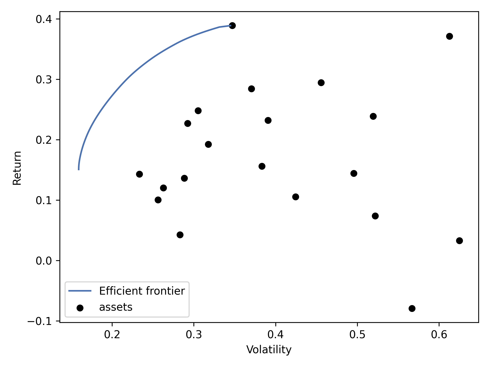
fig, ax = plt.subplots()
plotting.plot_efficient_frontier(ef, ax=ax, show_assets=True)
plt.show()
This produces the following plot:
You can explicitly pass a range of parameters (risk, utility, or returns) to generate a frontier:
# 100 portfolios with risks between 0.10 and 0.30
risk_range = np.linspace(0.10, 0.40, 100)
plotting.plot_efficient_frontier(ef, ef_param="risk", ef_param_range=risk_range,
                                show_assets=True, showfig=True)
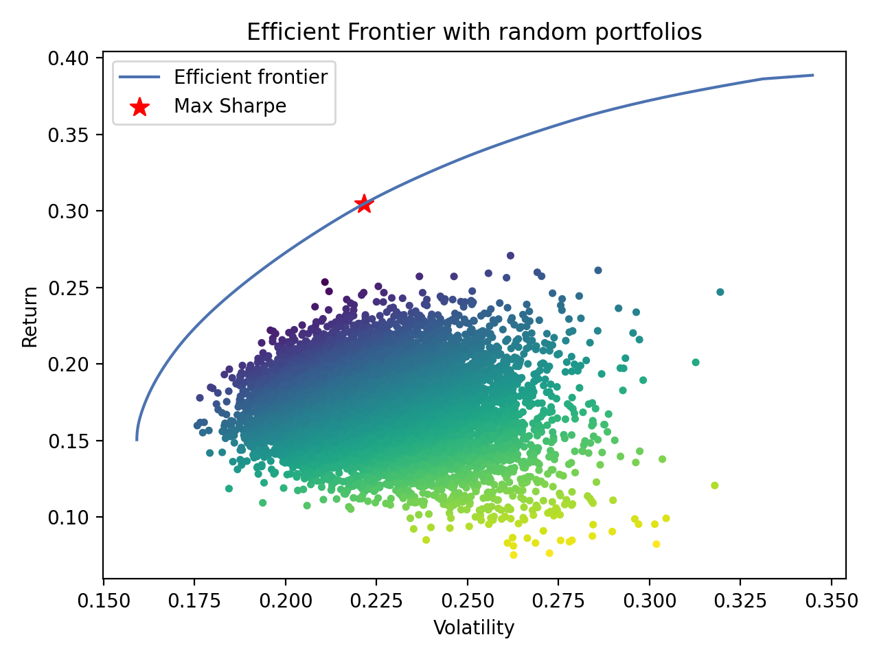
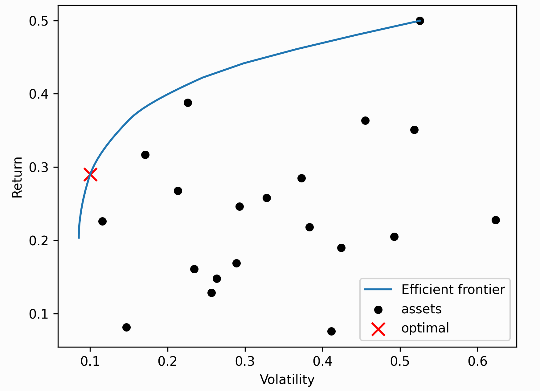
We can easily generate more complex plots. The following script plots both the efficient frontier and randomly generated (suboptimal) portfolios, coloured by the Sharpe ratio:
fig, ax = plt.subplots()
plotting.plot_efficient_frontier(ef, ax=ax, show_assets=False)

# Find the tangency portfolio
ef.max_sharpe()
ret_tangent, std_tangent, _ = ef.portfolio_performance()
ax.scatter(std_tangent, ret_tangent, marker="*", s=100, c="r", label="Max Sharpe")

# Generate random portfolios
n_samples = 10000
w = np.random.dirichlet(np.ones(len(mu)), n_samples)
rets = w.dot(mu)
stds = np.sqrt(np.diag(w @ S @ w.T))
sharpes = rets / stds
ax.scatter(stds, rets, marker=".", c=sharpes, cmap="viridis_r")

# Output
ax.set_title("Efficient Frontier with random portfolios")
ax.legend()
plt.tight_layout()
plt.savefig("ef_scatter.png", dpi=200)
plt.show()
This is the result:
Documentation reference
The plotting module houses all the functions to generate various plots.
Currently implemented:
plot_covariance- plot a correlation matrixplot_dendrogram- plot the hierarchical clusters in a portfolioplot_efficient_frontier– plot the efficient frontier from an EfficientFrontier or CLA objectplot_weights- bar chart of weights
Tip
To save the plot, pass filename="somefile.png" as a keyword argument to any of
the plotting functions. This (along with some other kwargs) get passed through
_plot_io() before being returned.
-
pypfopt.plotting._plot_io(**kwargs)[source]¶ Helper method to optionally save the figure to file.
Parameters: - filename (str, optional) – name of the file to save to, defaults to None (doesn’t save)
- dpi (int (between 50-500)) – dpi of figure to save or plot, defaults to 300
- showfig (bool, optional) – whether to plt.show() the figure, defaults to False
-
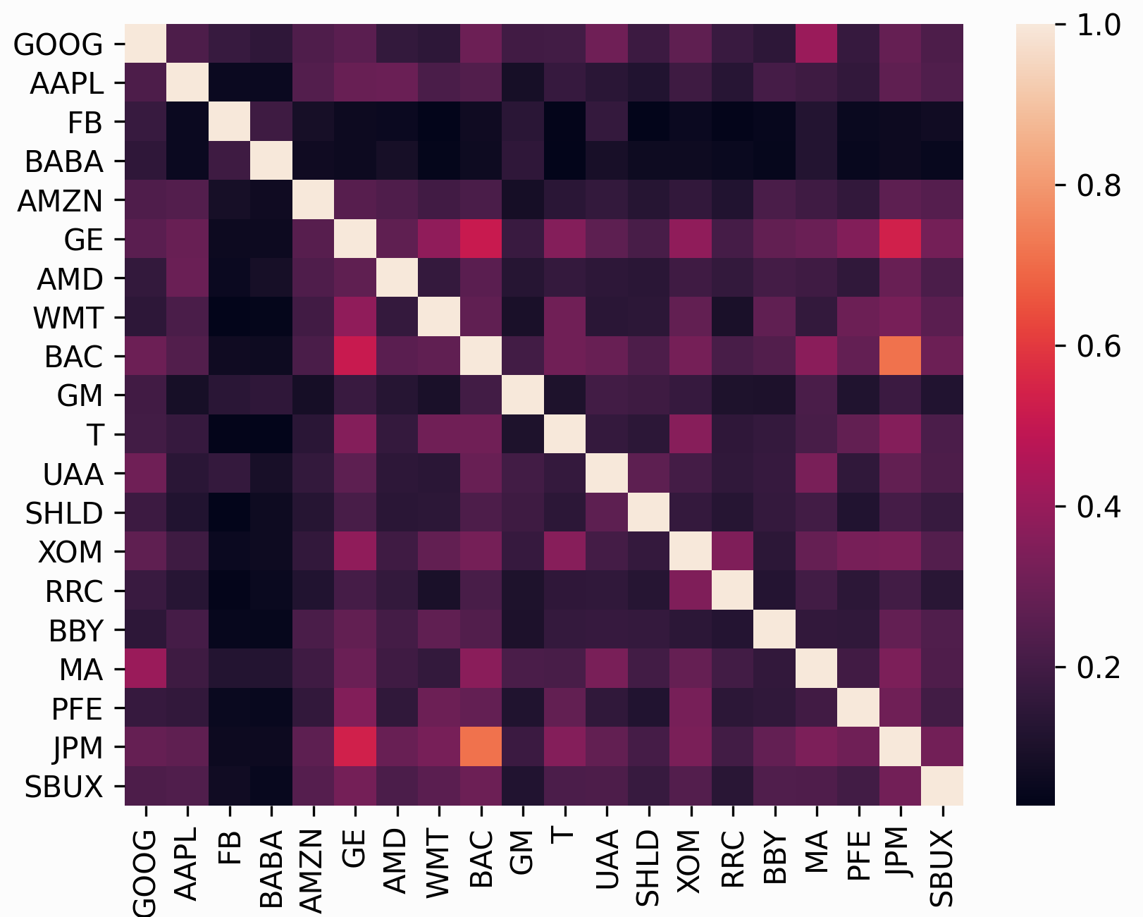
pypfopt.plotting.plot_covariance(cov_matrix, plot_correlation=False, show_tickers=True, **kwargs)[source]¶ Generate a basic plot of the covariance (or correlation) matrix, given a covariance matrix.
Parameters: - cov_matrix (pd.DataFrame or np.ndarray) – covariance matrix
- plot_correlation (bool, optional) – whether to plot the correlation matrix instead, defaults to False.
- show_tickers (bool, optional) – whether to use tickers as labels (not recommended for large portfolios), defaults to True
Returns: matplotlib axis
Return type: matplotlib.axes object
-
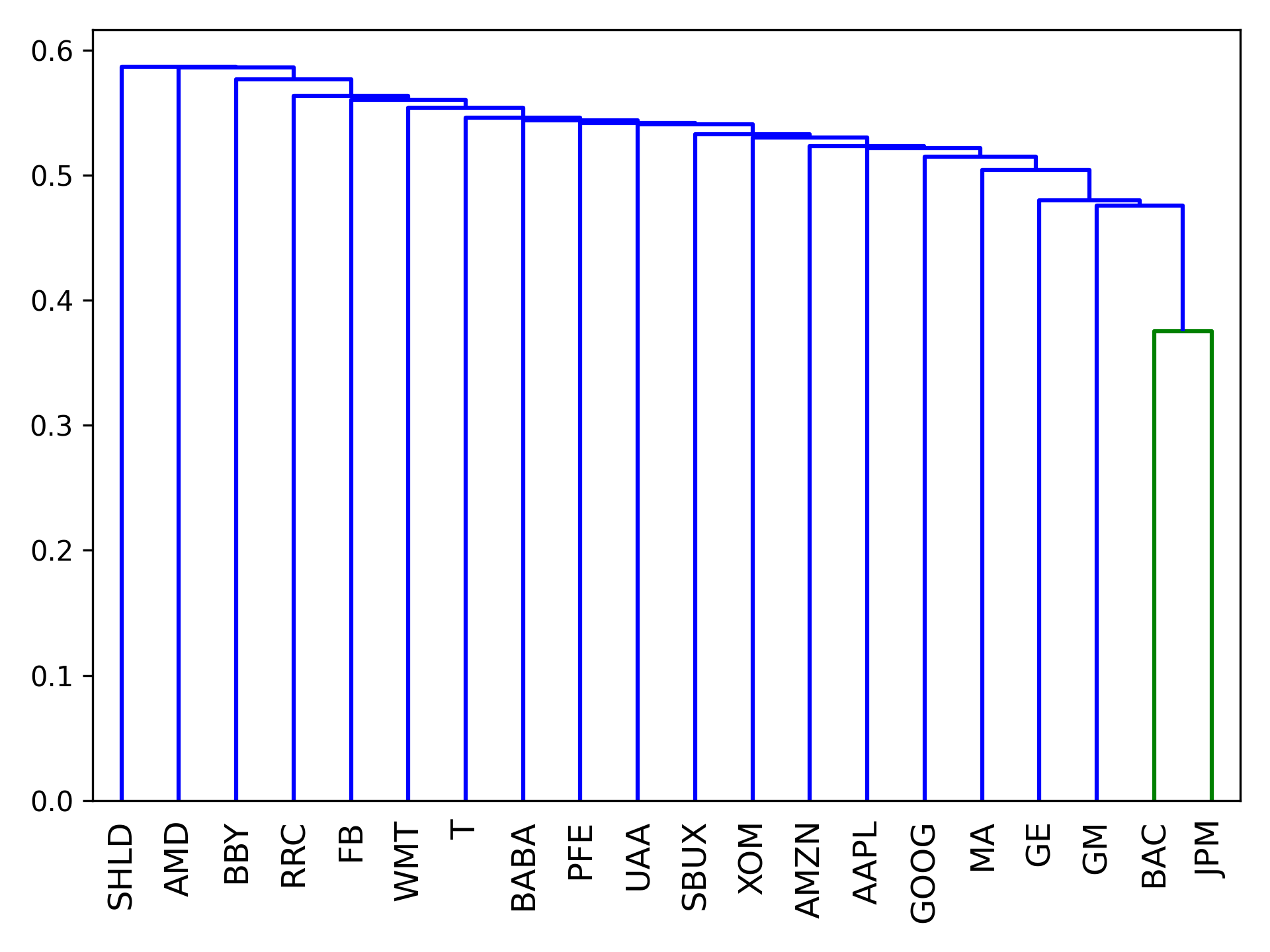
pypfopt.plotting.plot_dendrogram(hrp, ax=None, show_tickers=True, **kwargs)[source]¶ Plot the clusters in the form of a dendrogram.
Parameters: - hrp (object) – HRPpt object that has already been optimized.
- show_tickers (bool, optional) – whether to use tickers as labels (not recommended for large portfolios), defaults to True
- filename (str, optional) – name of the file to save to, defaults to None (doesn’t save)
- showfig (bool, optional) – whether to plt.show() the figure, defaults to False
Returns: matplotlib axis
Return type: matplotlib.axes object
-
pypfopt.plotting.plot_efficient_frontier(opt, ef_param='return', ef_param_range=None, points=100, ax=None, show_assets=True, **kwargs)[source]¶ Plot the efficient frontier based on either a CLA or EfficientFrontier object.
Parameters: - opt (EfficientFrontier or CLA) – an instantiated optimizer object BEFORE optimising an objective
- ef_param (str, one of {"utility", "risk", "return"}.) – [EfficientFrontier] whether to use a range over utility, risk, or return. Defaults to “return”.
- ef_param_range (np.array or list (recommended to use np.arange or np.linspace)) – the range of parameter values for ef_param. If None, automatically compute a range from min->max return.
- points (int, optional) – number of points to plot, defaults to 100. This is overridden if an ef_param_range is provided explicitly.
- show_assets (bool, optional) – whether we should plot the asset risks/returns also, defaults to True
- filename (str, optional) – name of the file to save to, defaults to None (doesn’t save)
- showfig (bool, optional) – whether to plt.show() the figure, defaults to False
Returns: matplotlib axis
Return type: matplotlib.axes object
-
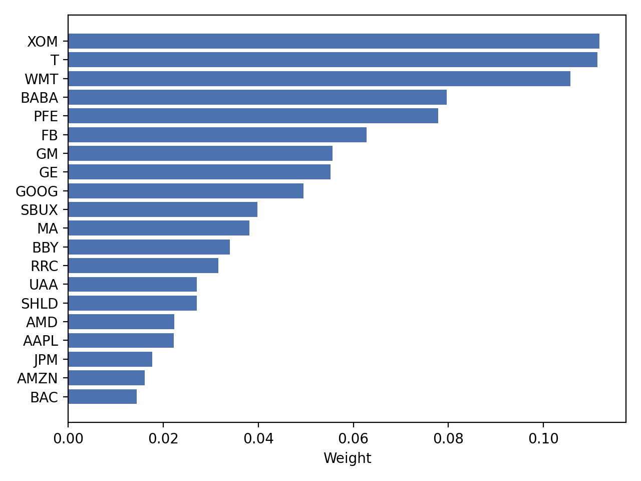
pypfopt.plotting.plot_weights(weights, ax=None, **kwargs)[source]¶ Plot the portfolio weights as a horizontal bar chart
Parameters: - weights ({ticker: weight} dict) – the weights outputted by any PyPortfolioOpt optimizer
- ax (matplotlib.axes) – ax to plot to, optional
Returns: matplotlib axis
Return type: matplotlib.axes