Risk Models

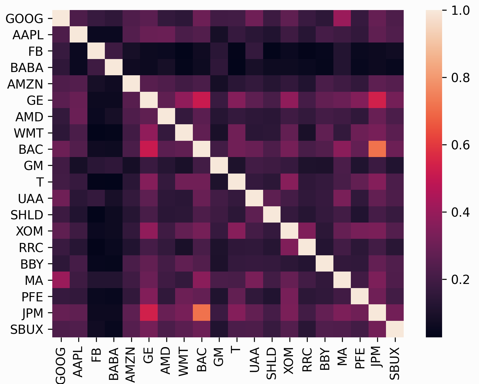
In addition to the expected returns, mean-variance optimization requires a risk model, some way of quantifying asset risk. The most commonly-used risk model is the covariance matrix, which describes asset volatilities and their co-dependence. This is important because one of the principles of diversification is that risk can be reduced by making many uncorrelated bets (correlation is just normalised covariance).

In many ways, the subject of risk models is far more important than that of expected returns because historical variance is generally a much more persistent statistic than mean historical returns. In fact, research by Kritzman et al. (2010) [1] suggests that minimum variance portfolios, formed by optimising without providing expected returns, actually perform much better out of sample.

The problem, however, is that in practice we do not have access to the covariance matrix (in the same way that we don’t have access to expected returns) – the only thing we can do is to make estimates based on past data. The most straightforward approach is to just calculate the sample covariance matrix based on historical returns, but relatively recent (post-2000) research indicates that there are much more robust statistical estimators of the covariance matrix. In addition to providing a wrapper around the estimators in sklearn, PyPortfolioOpt provides some experimental alternatives such as semicovariance and exponentially weighted covariance.

Attention

Estimation of the covariance matrix is a very deep and actively-researched topic that involves statistics, econometrics, and numerical/computational approaches. PyPortfolioOpt implements several options, but there is a lot of room for more sophistication.

The risk_models module provides functions for estimating the covariance matrix given historical returns.

The format of the data input is the same as that in Expected Returns.

Currently implemented:

• fix non-positive semidefinite matrices

• general risk matrix function, allowing you to run any risk model from one function.

• sample covariance

• semicovariance

• exponentially weighted covariance

• minimum covariance determinant

• shrunk covariance matrices:

  • manual shrinkage
  • Ledoit Wolf shrinkage
  • Oracle Approximating shrinkage

• covariance to correlation matrix

Note

For any of these methods, if you would prefer to pass returns (the default is prices), set the boolean flag returns_data=True

pypfopt.risk_models.risk_matrix(prices, method='sample_cov', **kwargs)

Compute a covariance matrix, using the risk model supplied in the method parameter.

Parameters:

• prices (pd.DataFrame) – adjusted closing prices of the asset, each row is a date and each column is a ticker/id.
• returns_data (bool, defaults to False.) – if true, the first argument is returns instead of prices.
• method (str, optional) –

  the risk model to use. Should be one of:

  • sample_cov
  • semicovariance
  • exp_cov
  • ledoit_wolf
  • ledoit_wolf_constant_variance
  • ledoit_wolf_single_factor
  • ledoit_wolf_constant_correlation
  • oracle_approximating

Raises:

NotImplementedError – if the supplied method is not recognised

Returns:

annualised sample covariance matrix

Return type:

pd.DataFrame

pypfopt.risk_models.fix_nonpositive_semidefinite(matrix, fix_method='spectral')

Check if a covariance matrix is positive semidefinite, and if not, fix it with the chosen method.

The spectral method sets negative eigenvalues to zero then rebuilds the matrix, while the diag method adds a small positive value to the diagonal.

Parameters:

• matrix (pd.DataFrame) – raw covariance matrix (may not be PSD)
• fix_method (str, optional) – {“spectral”, “diag”}, defaults to “spectral”

Raises:

NotImplementedError – if a method is passed that isn’t implemented

Returns:

positive semidefinite covariance matrix

Return type:

pd.DataFrame

Not all the calculated covariance matrices will be positive semidefinite (PSD). This method checks if a matrix is PSD and fixes it if not.

pypfopt.risk_models.sample_cov(prices, returns_data=False, frequency=252, **kwargs)

Calculate the annualised sample covariance matrix of (daily) asset returns.

Parameters:

• prices (pd.DataFrame) – adjusted closing prices of the asset, each row is a date and each column is a ticker/id.
• returns_data (bool, defaults to False.) – if true, the first argument is returns instead of prices.
• frequency (int, optional) – number of time periods in a year, defaults to 252 (the number of trading days in a year)

Returns:

annualised sample covariance matrix

Return type:

pd.DataFrame

This is the textbook default approach. The entries in the sample covariance matrix (which we denote as S) are the sample covariances between the i th and j th asset (the diagonals consist of variances). Although the sample covariance matrix is an unbiased estimator of the covariance matrix, i.e \(E(S) = \Sigma\), in practice it suffers from misspecification error and a lack of robustness. This is particularly problematic in mean-variance optimization, because the optimizer may give extra credence to the erroneous values.

Note

This should not be your default choice! Please use a shrinkage estimator instead.

pypfopt.risk_models.semicovariance(prices, returns_data=False, benchmark=7.9e-05, frequency=252, **kwargs)

Estimate the semicovariance matrix, i.e the covariance given that the returns are less than the benchmark.

Parameters:

• prices (pd.DataFrame) – adjusted closing prices of the asset, each row is a date and each column is a ticker/id.
• returns_data (bool, defaults to False.) – if true, the first argument is returns instead of prices.
• benchmark (float) – the benchmark return, defaults to the daily risk-free rate, i.e \(1.02^{(1/252)} -1\).
• frequency (int, optional) – number of time periods in a year, defaults to 252 (the number of trading days in a year). Ensure that you use the appropriate benchmark, e.g if frequency=12 use the monthly risk-free rate.

Returns:

semicovariance matrix

Return type:

pd.DataFrame

The semivariance is the variance of all returns which are below some benchmark B (typically the risk-free rate) – it is a common measure of downside risk. There are multiple possible ways of defining a semicovariance matrix, the main differences lying in the ‘pairwise’ nature, i.e whether we should sum over \(\min(r_i,B)\min(r_j,B)\) or \(\min(r_ir_j, B)\). In this implementation, we have followed the advice of Estrada (2007) [2], preferring:

\[\frac{1}{n}\sum_{i = 1}^n {\sum_{j = 1}^n {\min \left( {{r_i},B} \right)} } \min \left( {{r_j},B} \right)\]

pypfopt.risk_models.exp_cov(prices, returns_data=False, span=180, frequency=252, **kwargs)

Estimate the exponentially-weighted covariance matrix, which gives greater weight to more recent data.

Parameters:

• prices (pd.DataFrame) – adjusted closing prices of the asset, each row is a date and each column is a ticker/id.
• returns_data (bool, defaults to False.) – if true, the first argument is returns instead of prices.
• span (int, optional) – the span of the exponential weighting function, defaults to 180
• frequency (int, optional) – number of time periods in a year, defaults to 252 (the number of trading days in a year)

Returns:

annualised estimate of exponential covariance matrix

Return type:

pd.DataFrame

The exponential covariance matrix is a novel way of giving more weight to recent data when calculating covariance, in the same way that the exponential moving average price is often preferred to the simple average price. For a full explanation of how this estimator works, please refer to the blog post on my academic website.

pypfopt.risk_models.cov_to_corr(cov_matrix)

Convert a covariance matrix to a correlation matrix.

Parameters:cov_matrix (pd.DataFrame) – covariance matrix Returns:correlation matrix Return type:pd.DataFrame

pypfopt.risk_models.corr_to_cov(corr_matrix, stdevs)

Convert a correlation matrix to a covariance matrix

Parameters:

• corr_matrix (pd.DataFrame) – correlation matrix
• stdevs (array-like) – vector of standard deviations

Returns:

covariance matrix

Return type:

pd.DataFrame

Shrinkage estimators

A great starting point for those interested in understanding shrinkage estimators is Honey, I Shrunk the Sample Covariance Matrix [3] by Ledoit and Wolf, which does a good job at capturing the intuition behind them – we will adopt the notation used therein. I have written a summary of this article, which is available on my website. A more rigorous reference can be found in Ledoit and Wolf (2001) [4].

The essential idea is that the unbiased but often poorly estimated sample covariance can be combined with a structured estimator \(F\), using the below formula (where \(\delta\) is the shrinkage constant):

\[\hat{\Sigma} = \delta F + (1-\delta) S\]

It is called shrinkage because it can be thought of as “shrinking” the sample covariance matrix towards the other estimator, which is accordingly called the shrinkage target. The shrinkage target may be significantly biased but has little estimation error. There are many possible options for the target, and each one will result in a different optimal shrinkage constant \(\delta\). PyPortfolioOpt offers the following shrinkage methods:

• Ledoit-Wolf shrinkage:

  • constant_variance shrinkage, i.e the target is the diagonal matrix with the mean of asset variances on the diagonals and zeroes elsewhere. This is the shrinkage offered by sklearn.LedoitWolf.
  • single_factor shrinkage. Based on Sharpe’s single-index model which effectively uses a stock’s beta to the market as a risk model. See Ledoit and Wolf 2001 [4].
  • constant_correlation shrinkage, in which all pairwise correlations are set to the average correlation (sample variances are unchanged). See Ledoit and Wolf 2003 [3]

• Oracle approximating shrinkage (OAS), invented by Chen et al. (2010) [5], which has a lower mean-squared error than Ledoit-Wolf shrinkage when samples are Gaussian or near-Gaussian.

Tip

For most use cases, I would just go with Ledoit Wolf shrinkage, as recommended by Quantopian in their lecture series on quantitative finance.

My implementations have been translated from the Matlab code on Michael Wolf’s webpage, with the help of xtuanta.

class pypfopt.risk_models.CovarianceShrinkage(prices, returns_data=False, frequency=252)

Provide methods for computing shrinkage estimates of the covariance matrix, using the sample covariance matrix and choosing the structured estimator to be an identity matrix multiplied by the average sample variance. The shrinkage constant can be input manually, though there exist methods (notably Ledoit Wolf) to estimate the optimal value.

Instance variables:

• X - pd.DataFrame (returns)
• S - np.ndarray (sample covariance matrix)
• delta - float (shrinkage constant)
• frequency - int

__init__(prices, returns_data=False, frequency=252)

Parameters:

• prices (pd.DataFrame) – adjusted closing prices of the asset, each row is a date and each column is a ticker/id.
• returns_data (bool, defaults to False.) – if true, the first argument is returns instead of prices.
• frequency (int, optional) – number of time periods in a year, defaults to 252 (the number of trading days in a year)

ledoit_wolf(shrinkage_target='constant_variance')

Calculate the Ledoit-Wolf shrinkage estimate for a particular shrinkage target.

Parameters:shrinkage_target (str, optional) – choice of shrinkage target, either constant_variance, single_factor or constant_correlation. Defaults to constant_variance. Raises:NotImplementedError – if the shrinkage_target is unrecognised Returns:shrunk sample covariance matrix Return type:np.ndarray

oracle_approximating()

Calculate the Oracle Approximating Shrinkage estimate

Returns:shrunk sample covariance matrix Return type:np.ndarray

shrunk_covariance(delta=0.2)

Shrink a sample covariance matrix to the identity matrix (scaled by the average sample variance). This method does not estimate an optimal shrinkage parameter, it requires manual input.

Parameters:delta (float, optional) – shrinkage parameter, defaults to 0.2. Returns:shrunk sample covariance matrix Return type:np.ndarray

References

[1]	Kritzman, Page & Turkington (2010) In defense of optimization: The fallacy of 1/N. Financial Analysts Journal, 66(2), 31-39.

[2]	Estrada (2006), Mean-Semivariance Optimization: A Heuristic Approach

[3]	(1, 2) Ledoit, O., & Wolf, M. (2003). Honey, I Shrunk the Sample Covariance Matrix The Journal of Portfolio Management, 30(4), 110–119. https://doi.org/10.3905/jpm.2004.110

[4]	(1, 2) Ledoit, O., & Wolf, M. (2001). Improved estimation of the covariance matrix of stock returns with an application to portfolio selection, 10, 603–621.

[5]	Chen et al. (2010), Shrinkage Algorithms for MMSE Covariance Estimation, IEEE Transactions on Signals Processing, 58(10), 5016-5029.