User Guide
This is designed to be a practical guide, mostly aimed at users who are interested in a quick way of optimally combining some assets (most likely stocks). However, when necessary I do introduce the required theory and also point out areas that may be suitable springboards for more advanced optimization techniques. Details about the parameters can be found in the respective documentation pages (please see the sidebar).
For this guide, we will be focusing on mean-variance optimization (MVO), which is what most people think of when they hear “portfolio optimization”. MVO forms the core of PyPortfolioOpt’s offering, though it should be noted that MVO comes in many flavours, which can have very different performance characteristics. Please refer to the sidebar to get a feeling for the possibilities, as well as the other optimization methods offered. But for now, we will continue with the standard Efficient Frontier.
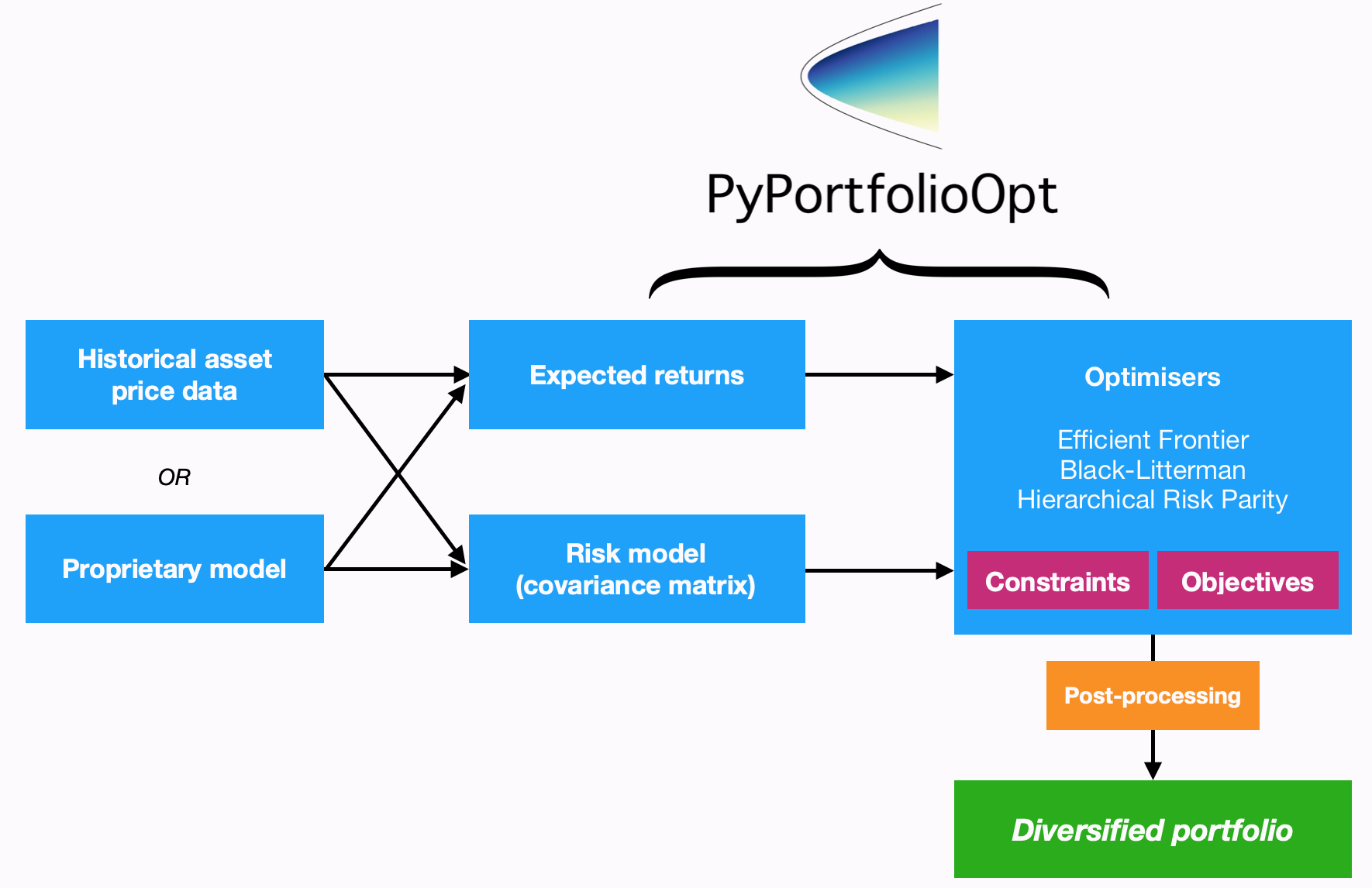
PyPortfolioOpt is designed with modularity in mind; the below flowchart sums up the current functionality and overall layout of PyPortfolioOpt.
Processing historical prices
Mean-variance optimization requires two things: the expected returns of the assets,
and the covariance matrix (or more generally, a risk model quantifying asset risk).
PyPortfolioOpt provides methods for estimating both (located in
expected_returns and risk_models respectively), but also supports
users who would like to use their own models.
However, I assume that most users will (at least initially) prefer to use the built-ins. In this case, all you need to supply is a dataset of historical prices for your assets. This dataset should look something like the one below:
                XOM        RRC        BBY         MA        PFE        JPM
date
2010-01-04  54.068794  51.300568  32.524055  22.062426  13.940202  35.175220
2010-01-05  54.279907  51.993038  33.349487  21.997149  13.741367  35.856571
2010-01-06  54.749043  51.690697  33.090542  22.081820  13.697187  36.053574
2010-01-07  54.577045  51.593170  33.616547  21.937523  13.645634  36.767757
2010-01-08  54.358093  52.597733  32.297466  21.945297  13.756095  36.677460
The index should consist of dates or timestamps, and each column should represent the time series of prices for an asset. A dataset of real-life stock prices has been included in the tests folder of the GitHub repo.
Note
Pricing data does not have to be daily, but the frequency should be the same across all assets (workarounds exist but are not pretty).
After reading your historical prices into a pandas dataframe df, you need to decide
between the available methods for estimating expected returns and the covariance matrix.
Sensible defaults are expected_returns.mean_historical_return() and
the Ledoit Wolf shrinkage estimate of the covariance matrix found in
risk_models.CovarianceShrinkage. It is simply a matter of applying the
relevant functions to the price dataset:
from pypfopt.expected_returns import mean_historical_return
from pypfopt.risk_models import CovarianceShrinkage

mu = mean_historical_return(df)
S = CovarianceShrinkage(df).ledoit_wolf()
mu will then be a pandas series of estimated expected returns for each asset,
and S will be the estimated covariance matrix (part of it is shown below):
        GOOG      AAPL        FB      BABA      AMZN        GE       AMD  \
GOOG  0.045529  0.022143  0.006389  0.003720  0.026085  0.015815  0.021761
AAPL  0.022143  0.207037  0.004334  0.002954  0.058200  0.038102  0.084053
FB    0.006389  0.004334  0.029233  0.003770  0.007619  0.003008  0.005804
BABA  0.003720  0.002954  0.003770  0.013438  0.004176  0.002011  0.006332
AMZN  0.026085  0.058200  0.007619  0.004176  0.276365  0.038169  0.075657
GE    0.015815  0.038102  0.003008  0.002011  0.038169  0.083405  0.048580
AMD   0.021761  0.084053  0.005804  0.006332  0.075657  0.048580  0.388916
Now that we have expected returns and a risk model, we are ready to move on to the actual portfolio optimization.
Mean-variance optimization
Mean-variance optimization is based on Harry Markowitz’s 1952 classic paper [1], which spearheaded the transformation of portfolio management from an art into a science. The key insight is that by combining assets with different expected returns and volatilities, one can decide on a mathematically optimal allocation.
If \(w\) is the weight vector of stocks with expected returns \(\mu\), then the portfolio return is equal to each stock’s weight multiplied by its return, i.e \(w^T \mu\). The portfolio risk in terms of the covariance matrix \(\Sigma\) is given by \(w^T \Sigma w\). Portfolio optimization can then be regarded as a convex optimization problem, and a solution can be found using quadratic programming. If we denote the target return as \(\mu^*\), the precise statement of the long-only portfolio optimization problem is as follows:
If we vary the target return, we will get a different set of weights (i.e a different portfolio) – the set of all these optimal portfolios is referred to as the efficient frontier.
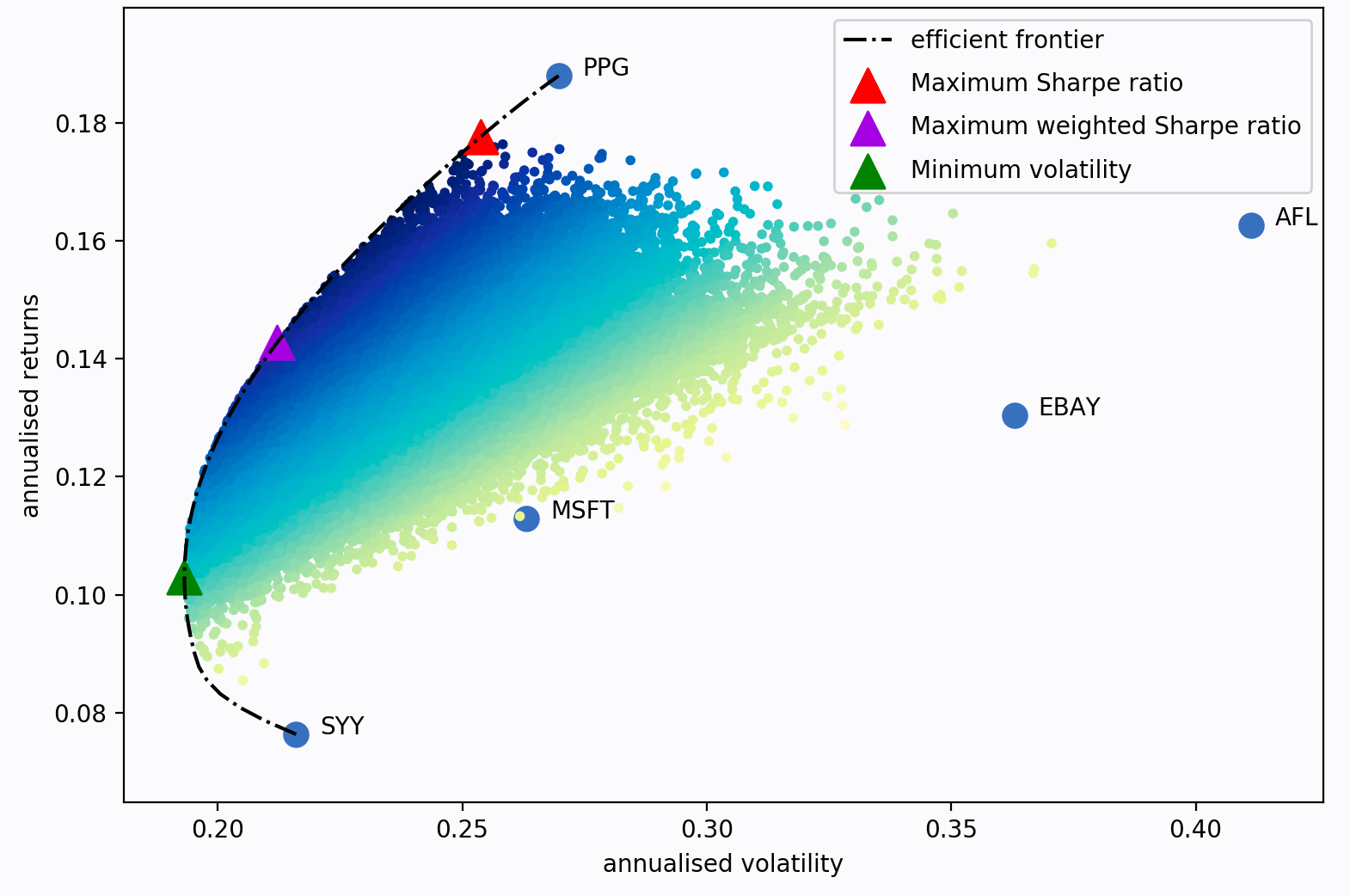
Each dot on this diagram represents a different possible portfolio, with darker blue corresponding to ‘better’ portfolios (in terms of the Sharpe Ratio). The dotted black line is the efficient frontier itself. The triangular markers represent the best portfolios for different optimization objectives.
The Sharpe ratio is the portfolio’s return in excess of the risk-free rate, per unit risk (volatility).
It is particularly important because it measures the portfolio returns, adjusted for
risk. So in practice, rather than trying to minimise volatility for a given target
return (as per Markowitz 1952), it often makes more sense to just find the portfolio
that maximises the Sharpe ratio. This is implemented as the max_sharpe()
method in the EfficientFrontier class. Using the series mu and
dataframe S from before:
from pypfopt.efficient_frontier import EfficientFrontier

ef = EfficientFrontier(mu, S)
weights = ef.max_sharpe()
If you print these weights, you will get quite an ugly result, because they will
be the raw output from the optimizer. As such, it is recommended that you use
the clean_weights() method, which truncates tiny weights to zero
and rounds the rest:
cleaned_weights = ef.clean_weights()
ef.save_weights_to_file("weights.txt")  # saves to file
print(cleaned_weights)
This prints:
{'GOOG': 0.01269,
'AAPL': 0.09202,
'FB': 0.19856,
'BABA': 0.09642,
'AMZN': 0.07158,
'GE': 0.0,
'AMD': 0.0,
'WMT': 0.0,
'BAC': 0.0,
'GM': 0.0,
'T': 0.0,
'UAA': 0.0,
'SHLD': 0.0,
'XOM': 0.0,
'RRC': 0.0,
'BBY': 0.06129,
'MA': 0.24562,
'PFE': 0.18413,
'JPM': 0.0,
'SBUX': 0.03769}
If we want to know the expected performance of the portfolio with optimal
weights w, we can use the portfolio_performance() method:
ef.portfolio_performance(verbose=True)
Expected annual return: 33.0%
Annual volatility: 21.7%
Sharpe Ratio: 1.43
A detailed discussion of optimization parameters is presented in General Efficient Frontier. However, there are two main variations which are discussed below.
Short positions
To allow for shorting, simply initialise the EfficientFrontier object
with bounds that allow negative weights, for example:
ef = EfficientFrontier(mu, S, weight_bounds=(-1,1))
This can be extended to generate market neutral portfolios (with weights
summing to zero), but these are only available for the efficient_risk()
and efficient_return() optimization methods for mathematical reasons.
If you want a market neutral portfolio, pass market_neutral=True as shown below:
ef.efficient_return(target_return=0.2, market_neutral=True)
Dealing with many negligible weights
From experience, I have found that mean-variance optimization often sets many of the asset weights to be zero. This may not be ideal if you need to have a certain number of positions in your portfolio, for diversification purposes or otherwise.
To combat this, I have introduced an objective function which borrows the idea of
regularisation from machine learning. Essentially, by adding an additional cost
function to the objective, you can ‘encourage’ the optimizer to choose different
weights (mathematical details are provided in the More on L2 Regularisation section).
To use this feature, change the gamma parameter:
from pypfopt import objective_functions

ef = EfficientFrontier(mu, S)
ef.add_objective(objective_functions.L2_reg, gamma=0.1)
w = ef.max_sharpe()
print(ef.clean_weights())
The result of this has far fewer negligible weights than before:
{'GOOG': 0.06366,
'AAPL': 0.09947,
'FB': 0.15742,
'BABA': 0.08701,
'AMZN': 0.09454,
'GE': 0.0,
'AMD': 0.0,
'WMT': 0.01766,
'BAC': 0.0,
'GM': 0.0,
'T': 0.00398,
'UAA': 0.0,
'SHLD': 0.0,
'XOM': 0.03072,
'RRC': 0.00737,
'BBY': 0.07572,
'MA': 0.1769,
'PFE': 0.12346,
'JPM': 0.0,
'SBUX': 0.06209}
Post-processing weights
In practice, we then need to convert these weights into an actual allocation, telling you how many shares of each asset you should purchase. This is discussed further in Post-processing weights, but we provide an example below:
from pypfopt.discrete_allocation import DiscreteAllocation, get_latest_prices

latest_prices = get_latest_prices(df)
da = DiscreteAllocation(w, latest_prices, total_portfolio_value=20000)
allocation, leftover = da.lp_portfolio()
print(allocation)
These are the quantities of shares that should be bought to have a $20,000 portfolio:
{'AAPL': 2.0,
'FB': 12.0,
'BABA': 14.0,
'GE': 18.0,
'WMT': 40.0,
'GM': 58.0,
'T': 97.0,
'SHLD': 1.0,
'XOM': 47.0,
'RRC': 3.0,
'BBY': 1.0,
'PFE': 47.0,
'SBUX': 5.0}
Improving performance
Let’s say you have conducted backtests and the results aren’t spectacular. What should you try?
- Try the Hierarchical Risk Parity model (see Other Optimizers) – which seems to robustly outperform mean-variance optimization out of sample.
- Use the Black-Litterman model to construct a more stable model of expected returns.
Alternatively, just drop the expected returns altogether! There is a large body of research
that suggests that minimum variance portfolios (
ef.min_volatility()) consistently outperform maximum Sharpe ratio portfolios out-of-sample (even when measured by Sharpe ratio), because of the difficulty of forecasting expected returns. - Try different risk models: shrinkage models are known to have better numerical properties compared with the sample covariance matrix.
- Add some new objective terms or constraints. Tune the L2 regularisation parameter to see how diversification affects the performance.
This concludes the guided tour. Head over to the appropriate sections in the sidebar to learn more about the parameters and theoretical details of the different models offered by PyPortfolioOpt. If you have any questions, please raise an issue on GitHub and I will try to respond promptly.
If you’d like even more examples, check out the cookbook recipe.
References
| [1] | Markowitz, H. (1952). Portfolio Selection. The Journal of Finance, 7(1), 77–91. https://doi.org/10.1111/j.1540-6261.1952.tb01525.x |