Other Optimizers
Efficient frontier methods involve the direct optimization of an objective subject to constraints. However, there are some portfolio optimization schemes that are completely different in character. PyPortfolioOpt provides support for these alternatives, while still giving you access to the same pre and post-processing API.
Note
As of v0.4, these other optimizers now inherit from BaseOptimizer or
BaseConvexOptimizer, so you no longer have to implement pre-processing and
post-processing methods on your own. You can thus easily swap out, say,
EfficientFrontier for HRPOpt.
Hierarchical Risk Parity (HRP)
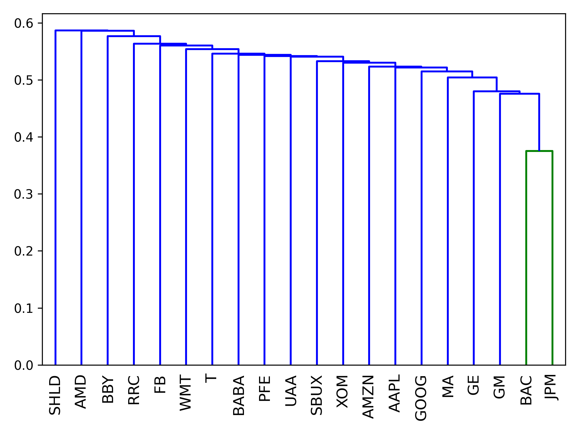
Hierarchical Risk Parity is a novel portfolio optimization method developed by Marcos Lopez de Prado [1]. Though a detailed explanation can be found in the linked paper, here is a rough overview of how HRP works:
- From a universe of assets, form a distance matrix based on the correlation of the assets.
- Using this distance matrix, cluster the assets into a tree via hierarchical clustering
- Within each branch of the tree, form the minimum variance portfolio (normally between just two assets).
- Iterate over each level, optimally combining the mini-portfolios at each node.
The advantages of this are that it does not require the inversion of the covariance matrix as with traditional mean-variance optimization, and seems to produce diverse portfolios that perform well out of sample.
The hierarchical_portfolio module seeks to implement one of the recent advances in
portfolio optimization – the application of hierarchical clustering models in allocation.
All of the hierarchical classes have a similar API to EfficientFrontier, though since
many hierarchical models currently don’t support different objectives, the actual allocation
happens with a call to optimize().
Currently implemented:
HRPOptimplements the Hierarchical Risk Parity (HRP) portfolio. Code reproduced with permission from Marcos Lopez de Prado (2016).
-
class
pypfopt.hierarchical_portfolio.HRPOpt(returns=None, cov_matrix=None)[source]¶ A HRPOpt object (inheriting from BaseOptimizer) constructs a hierarchical risk parity portfolio.
Instance variables:
Inputs
n_assets- inttickers- str listreturns- pd.DataFrame
Output:
weights- np.ndarrayclusters- linkage matrix corresponding to clustered assets.
Public methods:
optimize()calculates weights using HRPportfolio_performance()calculates the expected return, volatility and Sharpe ratio for the optimized portfolio.set_weights()creates self.weights (np.ndarray) from a weights dictclean_weights()rounds the weights and clips near-zeros.save_weights_to_file()saves the weights to csv, json, or txt.
-
__init__(returns=None, cov_matrix=None)[source]¶ Parameters: - returns (pd.DataFrame) – asset historical returns
- cov_matrix (pd.DataFrame.) – covariance of asset returns
Raises: TypeError – if
returnsis not a dataframe
-
optimize(linkage_method='single')[source]¶ Construct a hierarchical risk parity portfolio, using Scipy hierarchical clustering (see here)
Parameters: linkage_method (str) – which scipy linkage method to use Returns: weights for the HRP portfolio Return type: OrderedDict
-
portfolio_performance(verbose=False, risk_free_rate=0.02, frequency=252)[source]¶ After optimising, calculate (and optionally print) the performance of the optimal portfolio. Currently calculates expected return, volatility, and the Sharpe ratio assuming returns are daily
Parameters: - verbose (bool, optional) – whether performance should be printed, defaults to False
- risk_free_rate (float, optional) – risk-free rate of borrowing/lending, defaults to 0.02. The period of the risk-free rate should correspond to the frequency of expected returns.
- frequency (int, optional) – number of time periods in a year, defaults to 252 (the number of trading days in a year)
Raises: ValueError – if weights have not been calculated yet
Returns: expected return, volatility, Sharpe ratio.
Return type: (float, float, float)
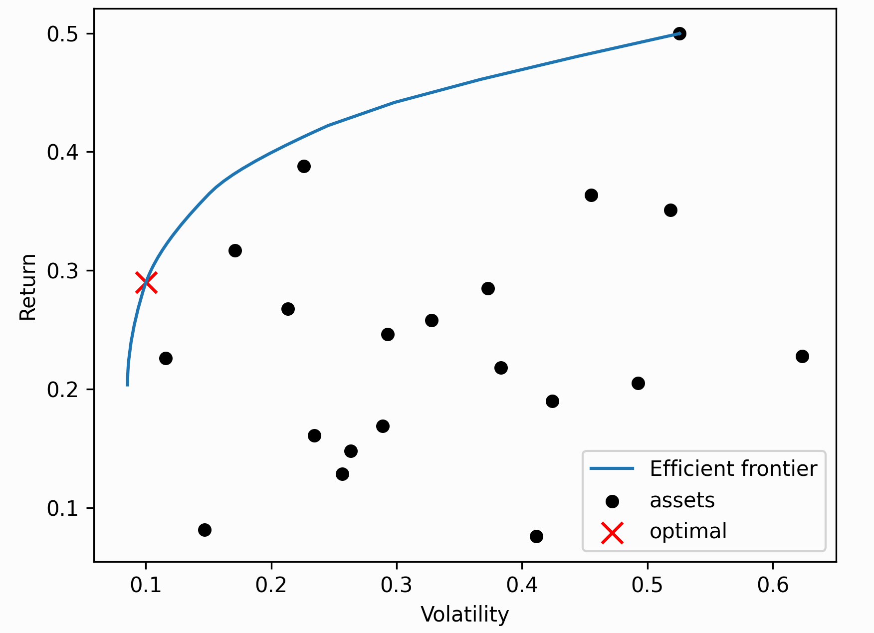
The Critical Line Algorithm
This is a robust alternative to the quadratic solver used to find mean-variance optimal portfolios, that is especially advantageous when we apply linear inequalities. Unlike generic convex optimization routines, the CLA is specially designed for portfolio optimization. It is guaranteed to converge after a certain number of iterations, and can efficiently derive the entire efficient frontier.
Tip
In general, unless you have specific requirements e.g you would like to efficiently compute the entire
efficient frontier for plotting, I would go with the standard EfficientFrontier optimizer.
I am most grateful to Marcos López de Prado and David Bailey for providing the implementation [2].
Permission for its distribution has been received by email. It has been modified such that it has
the same API, though as of v0.5.0 we only support max_sharpe() and min_volatility().
The cla module houses the CLA class, which
generates optimal portfolios using the Critical Line Algorithm as implemented
by Marcos Lopez de Prado and David Bailey.
-
class
pypfopt.cla.CLA(expected_returns, cov_matrix, weight_bounds=(0, 1))[source]¶ Instance variables:
Inputs:
n_assets- inttickers- str listmean- np.ndarraycov_matrix- np.ndarrayexpected_returns- np.ndarraylb- np.ndarrayub- np.ndarray
Optimization parameters:
w- np.ndarray listls- float listg- float listf- float list list
Outputs:
weights- np.ndarrayfrontier_values- (float list, float list, np.ndarray list)
Public methods:
max_sharpe()optimizes for maximal Sharpe ratio (a.k.a the tangency portfolio)min_volatility()optimizes for minimum volatilityefficient_frontier()computes the entire efficient frontierportfolio_performance()calculates the expected return, volatility and Sharpe ratio for the optimized portfolio.clean_weights()rounds the weights and clips near-zeros.save_weights_to_file()saves the weights to csv, json, or txt.
-
__init__(expected_returns, cov_matrix, weight_bounds=(0, 1))[source]¶ Parameters: - expected_returns (pd.Series, list, np.ndarray) – expected returns for each asset. Set to None if optimising for volatility only.
- cov_matrix (pd.DataFrame or np.array) – covariance of returns for each asset
- weight_bounds (tuple (float, float) or (list/ndarray, list/ndarray) or list(tuple(float, float))) – minimum and maximum weight of an asset, defaults to (0, 1). Must be changed to (-1, 1) for portfolios with shorting.
Raises: - TypeError – if
expected_returnsis not a series, list or array - TypeError – if
cov_matrixis not a dataframe or array
-
efficient_frontier(points=100)[source]¶ Efficiently compute the entire efficient frontier
Parameters: points (int, optional) – rough number of points to evaluate, defaults to 100 Raises: ValueError – if weights have not been computed Returns: return list, std list, weight list Return type: (float list, float list, np.ndarray list)
-
max_sharpe()[source]¶ Maximise the Sharpe ratio.
Returns: asset weights for the max-sharpe portfolio Return type: OrderedDict
-
min_volatility()[source]¶ Minimise volatility.
Returns: asset weights for the volatility-minimising portfolio Return type: OrderedDict
-
portfolio_performance(verbose=False, risk_free_rate=0.02)[source]¶ After optimising, calculate (and optionally print) the performance of the optimal portfolio. Currently calculates expected return, volatility, and the Sharpe ratio.
Parameters: - verbose (bool, optional) – whether performance should be printed, defaults to False
- risk_free_rate (float, optional) – risk-free rate of borrowing/lending, defaults to 0.02
Raises: ValueError – if weights have not been calculated yet
Returns: expected return, volatility, Sharpe ratio.
Return type: (float, float, float)
Implementing your own optimizer
Please note that this is quite different to implementing Custom optimization problems, because in that case we are still using the same convex optimization structure. However, HRP and CLA optimization have a fundamentally different optimization method. In general, these are much more difficult to code up compared to custom objective functions.
To implement a custom optimizer that is compatible with the rest of PyPortfolioOpt, just
extend BaseOptimizer (or BaseConvexOptimizer if you want to use cvxpy),
both of which can be found in base_optimizer.py. This gives you access to utility
methods like clean_weights(), as well as making sure that any output is compatible
with portfolio_performance() and post-processing methods.
The base_optimizer module houses the parent classes BaseOptimizer from which all
optimizers will inherit. BaseConvexOptimizer is the base class for all cvxpy (and scipy)
optimization.
Additionally, we define a general utility function portfolio_performance to
evaluate return and risk for a given set of portfolio weights.
-
class
pypfopt.base_optimizer.BaseOptimizer(n_assets, tickers=None)[source]¶ Instance variables:
n_assets- inttickers- str listweights- np.ndarray
Public methods:
set_weights()creates self.weights (np.ndarray) from a weights dictclean_weights()rounds the weights and clips near-zeros.save_weights_to_file()saves the weights to csv, json, or txt.
-
__init__(n_assets, tickers=None)[source]¶ Parameters: - n_assets (int) – number of assets
- tickers (list) – name of assets
-
clean_weights(cutoff=0.0001, rounding=5)[source]¶ Helper method to clean the raw weights, setting any weights whose absolute values are below the cutoff to zero, and rounding the rest.
Parameters: - cutoff (float, optional) – the lower bound, defaults to 1e-4
- rounding (int, optional) – number of decimal places to round the weights, defaults to 5. Set to None if rounding is not desired.
Returns: asset weights
Return type: OrderedDict
-
class
pypfopt.base_optimizer.BaseConvexOptimizer(n_assets, tickers=None, weight_bounds=(0, 1), solver=None, verbose=False, solver_options=None)[source]¶ The BaseConvexOptimizer contains many private variables for use by
cvxpy. For example, the immutable optimization variable for weights is stored as self._w. Interacting directly with these variables directly is discouraged.Instance variables:
n_assets- inttickers- str listweights- np.ndarray_opt- cp.Problem_solver- str_solver_options- {str: str} dict
Public methods:
add_objective()adds a (convex) objective to the optimization problemadd_constraint()adds a constraint to the optimization problemconvex_objective()solves for a generic convex objective with linear constraintsnonconvex_objective()solves for a generic nonconvex objective using the scipy backend. This is prone to getting stuck in local minima and is generally not recommended.set_weights()creates self.weights (np.ndarray) from a weights dictclean_weights()rounds the weights and clips near-zeros.save_weights_to_file()saves the weights to csv, json, or txt.
-
__init__(n_assets, tickers=None, weight_bounds=(0, 1), solver=None, verbose=False, solver_options=None)[source]¶ Parameters: - weight_bounds (tuple OR tuple list, optional) – minimum and maximum weight of each asset OR single min/max pair if all identical, defaults to (0, 1). Must be changed to (-1, 1) for portfolios with shorting.
- solver (str, optional.) – name of solver. list available solvers with:
cvxpy.installed_solvers() - verbose (bool, optional) – whether performance and debugging info should be printed, defaults to False
- solver_options (dict, optional) – parameters for the given solver
-
_map_bounds_to_constraints(test_bounds)[source]¶ Convert input bounds into a form acceptable by cvxpy and add to the constraints list.
Parameters: test_bounds (tuple OR list/tuple of tuples OR pair of np arrays) – minimum and maximum weight of each asset OR single min/max pair if all identical OR pair of arrays corresponding to lower/upper bounds. defaults to (0, 1). Raises: TypeError – if test_boundsis not of the right typeReturns: bounds suitable for cvxpy Return type: tuple pair of np.ndarray
-
_solve_cvxpy_opt_problem()[source]¶ Helper method to solve the cvxpy problem and check output, once objectives and constraints have been defined
Raises: exceptions.OptimizationError – if problem is not solvable by cvxpy
-
add_constraint(new_constraint)[source]¶ Add a new constraint to the optimization problem. This constraint must satisfy DCP rules, i.e be either a linear equality constraint or convex inequality constraint.
Examples:
ef.add_constraint(lambda x : x[0] == 0.02)
ef.add_constraint(lambda x : x >= 0.01)
ef.add_constraint(lambda x: x <= np.array([0.01, 0.08, ..., 0.5]))
Parameters: new_constraint (callable (e.g lambda function)) – the constraint to be added
-
add_objective(new_objective, **kwargs)[source]¶ Add a new term into the objective function. This term must be convex, and built from cvxpy atomic functions.
Example:
def L1_norm(w, k=1):
    return k * cp.norm(w, 1)

ef.add_objective(L1_norm, k=2)
Parameters: new_objective (cp.Expression (i.e function of cp.Variable)) – the objective to be added
-
add_sector_constraints(sector_mapper, sector_lower, sector_upper)[source]¶ Adds constraints on the sum of weights of different groups of assets. Most commonly, these will be sector constraints e.g portfolio’s exposure to tech must be less than x%:
sector_mapper = {
    "GOOG": "tech",
    "FB": "tech",,
    "XOM": "Oil/Gas",
    "RRC": "Oil/Gas",
    "MA": "Financials",
    "JPM": "Financials",
}

sector_lower = {"tech": 0.1}  # at least 10% to tech
sector_upper = {
    "tech": 0.4, # less than 40% tech
    "Oil/Gas": 0.1 # less than 10% oil and gas
}
Parameters: - sector_mapper ({str: str} dict) – dict that maps tickers to sectors
- sector_lower ({str: float} dict) – lower bounds for each sector
- sector_upper ({str:float} dict) – upper bounds for each sector
-
convex_objective(custom_objective, weights_sum_to_one=True, **kwargs)[source]¶ Optimize a custom convex objective function. Constraints should be added with
ef.add_constraint(). Optimizer arguments must be passed as keyword-args. Example:# Could define as a lambda function instead def logarithmic_barrier(w, cov_matrix, k=0.1): # 60 Years of Portfolio Optimization, Kolm et al (2014) return cp.quad_form(w, cov_matrix) - k * cp.sum(cp.log(w)) w = ef.convex_objective(logarithmic_barrier, cov_matrix=ef.cov_matrix)
Parameters: - custom_objective (function with signature (cp.Variable, **kwargs) -> cp.Expression) – an objective function to be MINIMISED. This should be written using cvxpy atoms Should map (w, **kwargs) -> float.
- weights_sum_to_one (bool, optional) – whether to add the default objective, defaults to True
Raises: OptimizationError – if the objective is nonconvex or constraints nonlinear.
Returns: asset weights for the efficient risk portfolio
Return type: OrderedDict
-
deepcopy()[source]¶ Returns a custom deep copy of the optimizer. This is necessary because
cvxpyexpressions do not support deepcopy, but the mutable arguments need to be copied to avoid unintended side effects. Instead, we create a shallow copy of the optimizer and then manually copy the mutable arguments.
-
nonconvex_objective(custom_objective, objective_args=None, weights_sum_to_one=True, constraints=None, solver='SLSQP', initial_guess=None)[source]¶ Optimize some objective function using the scipy backend. This can support nonconvex objectives and nonlinear constraints, but may get stuck at local minima. Example:
# Market-neutral efficient risk
constraints = [
    {"type": "eq", "fun": lambda w: np.sum(w)},  # weights sum to zero
    {
        "type": "eq",
        "fun": lambda w: target_risk ** 2 - np.dot(w.T, np.dot(ef.cov_matrix, w)),
    },  # risk = target_risk
]
ef.nonconvex_objective(
    lambda w, mu: -w.T.dot(mu),  # min negative return (i.e maximise return)
    objective_args=(ef.expected_returns,),
    weights_sum_to_one=False,
    constraints=constraints,
)
Parameters: - objective_function (function with signature (np.ndarray, args) -> float) – an objective function to be MINIMISED. This function should map (weight, args) -> cost
- objective_args (tuple of np.ndarrays) – arguments for the objective function (excluding weight)
- weights_sum_to_one (bool, optional) – whether to add the default objective, defaults to True
- constraints (dict list) – list of constraints in the scipy format (i.e dicts)
- solver (string) – which SCIPY solver to use, e.g “SLSQP”, “COBYLA”, “BFGS”. User beware: different optimizers require different inputs.
- initial_guess (np.ndarray) – the initial guess for the weights, shape (n,) or (n, 1)
Returns: asset weights that optimize the custom objective
Return type: OrderedDict
References
| [1] | López de Prado, M. (2016). Building Diversified Portfolios that Outperform Out of Sample. The Journal of Portfolio Management, 42(4), 59–69. |
| [2] | Bailey and Loópez de Prado (2013). An Open-Source Implementation of the Critical-Line Algorithm for Portfolio Optimization |